Modeling a Speculative Asteroid Value Target with Public Data

Overview

I have a geology background, so I have always been drawn to questions about what things are made of, how they formed, and what their physical properties can reveal. Once I started looking at asteroid data through that lens, it felt like a natural place to combine that interest with coding.

At some point that curiosity turned into a project. I started pulling public asteroid data, cleaning it up, mapping spectral classes to rough composition priors, and building a small machine learning pipeline around a speculative value target. It was one of those projects where the initial question was simple enough to get moving, but every step opened up a deeper one behind it.

The project itself was exciting because it gave me something tangible: a real dataset, engineered features, trained models, saved artifacts, and a few visualizations that told a story. But looking back on it now, what stands out more is what it revealed about how I was learning. I had moved quickly from curiosity to implementation, but not always from curiosity to understanding.

That is really what this post is about. First, I want to walk through the pipeline I built and the assumptions it depended on. Then I want to explain why that process convinced me to go back and build a stronger foundation in physics and machine learning instead of relying on AI to help me assemble systems I could not yet fully explain on my own.

Why I Built This

A pipe dream of mine is to one day be part of a team building swarms of tiny spacecraft that can analyze asteroids in the asteroid belt. Do I think that is feasible in my lifetime? Probably not. But I do think it is an exciting idea, and I want to be part of the conversation around it.

This project was a way to start pulling that idea down to earth. I wanted to see what I could learn from public asteroid data, what kinds of features might matter, and how far I could get by building a small pipeline around a speculative value target.

Part of the experiment was also seeing how far I could get with AI helping me move quickly. I was able to assemble a real pipeline faster than I would have otherwise, but revisiting it later made me realize there is a big difference between building something and fully understanding it.

That realization is a big part of why this project matters to me now: it gave me something concrete to build, but it also showed me exactly what I still want to understand more deeply.

The Project at a Glance

At a high level, this project was an end-to-end experiment built around public asteroid data from Asterank. The workflow looked like this:

1. Scrape asteroid records from the Asterank API
2. Save the raw dataset locally
3. Clean and process the data into a more usable table
4. Add composition-based features using asteroid spectral class as a proxy
5. Engineer a small set of additional features related to size, orbit, and material composition
6. Train regression models to predict a speculative value target
7. Visualize the results to better understand the data and tell the story

The target in this case was not a scientifically rigorous measure of economic value. It was a speculative value field already present in the public dataset, which made the project more of a modeling exercise around a proxy target than a serious valuation system. Still, it was a useful way to think through how asteroid composition, orbital properties, and observability might show up in a modeling pipeline.

For the modeling step, I trained a Random Forest regressor and an XGBoost regressor, then compared their outputs and feature importances.

Collecting the Data

The project started with public asteroid data from the Asterank API. It is a great free source of asteroid records and includes a wide range of physical and orbital properties. One practical issue, though, is that the API does not support pagination. Since each request is limited to 1000 results, I needed a way to collect a larger slice of the dataset without just accepting whatever happened to fit into a single query.

My solution was to query the API in diameter bins. Smaller bins helped in denser parts of the dataset, while larger bins were enough for sparser ranges. That gave me a way to pull the data incrementally without exceeding the request limit, while also making the collection process easier to reason about. Most of the dataset was concentrated at the small-diameter end of the distribution, so that was the part most likely to overflow the API limit.

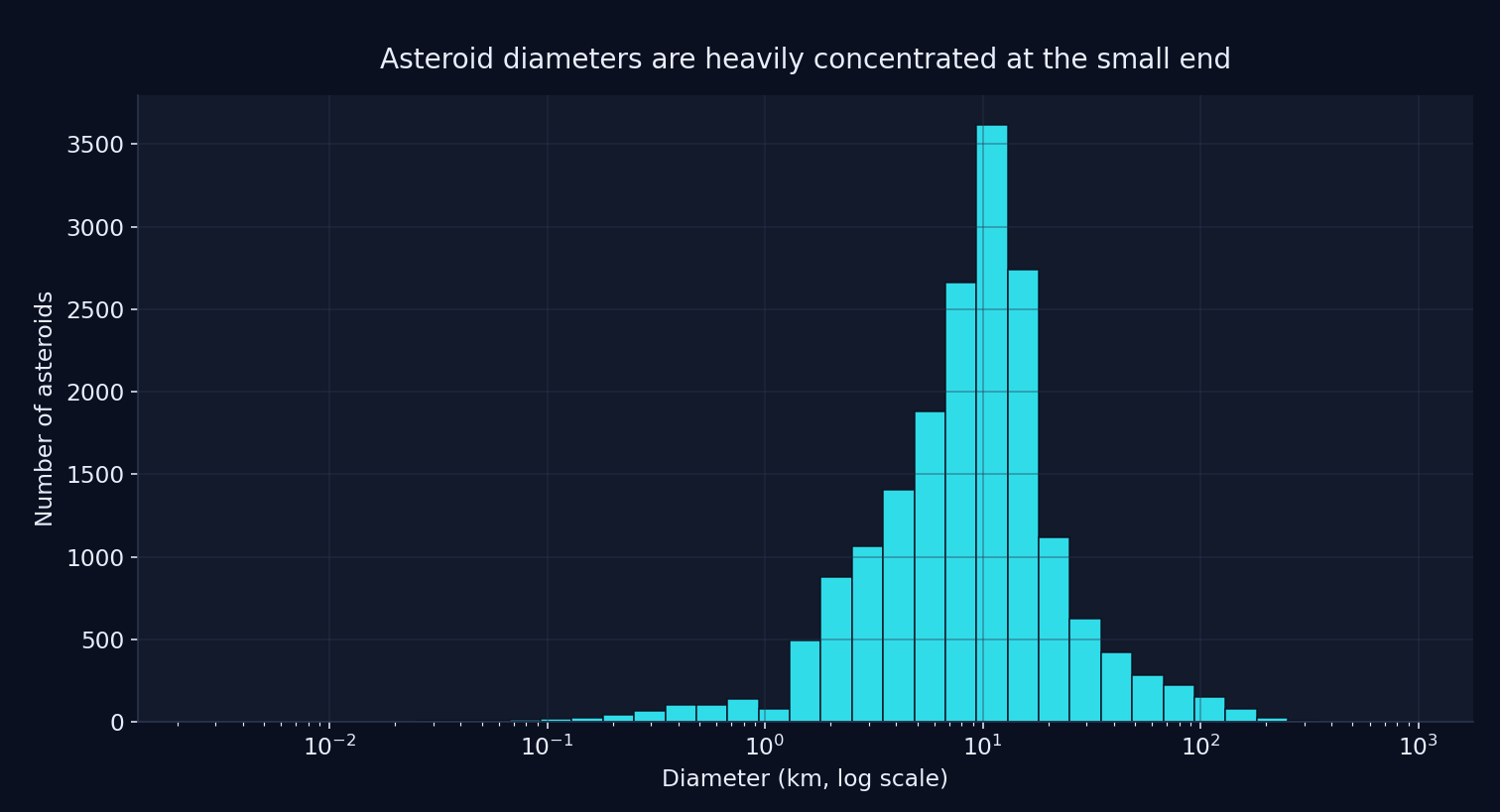
Asteroid diameters on a log-scaled x-axis. The distribution is heavily concentrated among smaller objects, which is why querying the API in smaller diameter bins mattered.

def fetch_asteroid_data():
    all_asteroids = []

    bin_ranges = [
        (0, 20, 1.0),
        (20, 100, 10.0),
        (100, 300, 50.0),
        (300, 1000, 700.0),
    ]

    for min_diameter, max_diameter, bin_size in bin_ranges:
        current_min = min_diameter

        while current_min < max_diameter:
            current_max = min(current_min + bin_size, max_diameter)
            query = f'{{"diameter": {{"$gt": {current_min}, "$lt": {current_max}}}}}'
            response = requests.get(API_URL.format(query))

            if response.status_code != 200:
                raise Exception(f"Error: {response.status_code}")

            data = response.json()
            if not data:
                break

            all_asteroids.extend(data)
            current_min = current_max
            time.sleep(1)

    return pd.DataFrame(all_asteroids)

Once I had accumulated the records, I sorted them by diameter and saved the raw results locally as a CSV. That gave me a clean separation between the ingestion step and the later cleaning, feature engineering, and modeling work.

Modeling a Speculative Value Target

The next important choice in the project was the target itself. I was not trying to predict any rigorous notion of real asteroid economic value. Instead, I used the price field already present in the Asterank data as a speculative value target.

That distinction matters. This project was never a serious attempt to estimate the real future market value of an asteroid or to model the economics of asteroid mining in any defensible way. It was an experiment built around a public dataset that already included a value field, plus my own feature engineering and composition-based assumptions.

In practice, that made the project more like a modeling exercise around a proxy target than a true valuation system. But that was still useful. It let me ask questions like: if I combine orbital features, size, and rough composition priors, can I build a model that captures some of the structure behind this speculative target?

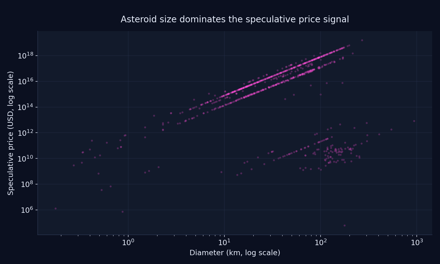
Diameter and speculative price plotted on log scales. Larger asteroids dominate the target by many orders of magnitude, while the visible banding suggests that size was not the only factor shaping the underlying pricing logic.

It also made the limitations of the project impossible to ignore. Any model I trained was only ever going to be as meaningful as the target it was learning from. In this case that target came with a lot of assumptions baked in before I touched the data at all.

From Spectral Class to Composition Proxies

Raw asteroid records gave me orbital and physical properties, but they did not directly give me the kind of material breakdown I was interested in. Since part of the question I cared about was whether different asteroids might be more or less interesting from a resource perspective, I wanted a way to represent composition more explicitly in the dataset.

My approach was to use each asteroid’s spectral class (spec) as a rough proxy for composition. I created a hand-built mapping from spectral classes to simplified material profiles, including things like iron, nickel, cobalt, water, and a few other components. For example, metal-rich classes got higher iron and nickel values, while carbonaceous classes got more weight on water and volatile-related features.

{
  "C": {
    "nickel": 0.014,
    "iron": 0.166,
    "cobalt": 0.002,
    "water": 0.2
  },
  "M": {
    "nickel": 10,
    "iron": 88,
    "cobalt": 0.5
  },
  "P": {
    "water": 12.5
  },
  "X": {
    "nickel": 10,
    "iron": 88,
    "cobalt": 0.5
  }
}

I then added this composition data as a new field and expanded it into separate columns for modeling. That made it possible to engineer additional features like total metal content, water-to-size ratio, and iron-to-nickel ratio.

This was also one of the most assumption-heavy parts of the entire pipeline. Spectral class is not the same thing as directly measured composition, and the mapping I used was more of a practical prior than a scientifically rigorous model. Still, it made the dataset much more interesting to work with and pushed the project closer to the kind of question I actually wanted to explore.

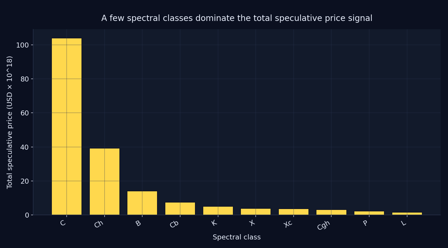
Summing the speculative price target by spectral class shows a highly concentrated distribution, with a small number of classes accounting for most of the aggregate signal in the dataset.

Feature Engineering

Once I had the raw data and composition proxies in place, the next step was to build features that might be useful for modeling the target. Some came directly from the source data, while others were simple combinations or ratios meant to capture something more interpretable about composition, orbit, or observability.

A few of the most important engineered features were:

• total_metal — combines estimated iron, nickel, and cobalt into a rough metal-content proxy.
• water_to_size_ratio — estimated water content normalized by asteroid diameter.
• e_to_a_ratio — combines eccentricity and semi-major axis into a compact orbital-shape feature.
• H_to_diameter_ratio — a rough brightness-to-size proxy based on absolute magnitude and diameter.
• rotational_energy_proxy — combines rotation period and diameter squared as a crude stand-in for rotational significance.
• observation_quality — uses number of observations, RMS error, and data arc as a rough measure of how well characterized an object is.
• orbit_stability — a simplified proxy based on semi-major axis, eccentricity, and inclination.
• neo_risk_factor — combines size and minimum orbit intersection distance.
• iron_to_nickel_ratio — captures composition mix in more detail than total metal alone.
• tisserand_parameter — a more physics-informed orbital feature drawn from classical orbital dynamics.

Some of these were more physically grounded than others. A few were straightforward material aggregates, while others were closer to heuristic proxies than formal scientific quantities.

Here is a small sample of the feature engineering logic:

dataset['total_metal'] = dataset['comp_iron'] + dataset['comp_nickel'] + dataset['comp_cobalt']
dataset['water_to_size_ratio'] = dataset['comp_water'] / dataset['diameter']
dataset['observation_quality'] = np.where(
    (dataset['rms'] != 0) & (dataset['data_arc'] != 0),
    dataset['n_obs_used'] / (dataset['rms'] * dataset['data_arc']),
    0
)
dataset['orbit_stability'] = dataset['a'] * (1 - dataset['e']) * np.cos(np.radians(dataset['i']))
dataset['iron_to_nickel_ratio'] = np.where(
    dataset['comp_nickel'] != 0,
    dataset['comp_iron'] / dataset['comp_nickel'],
    0
)

Training the Models

Once the dataset was in a shape I liked, the modeling step itself was fairly straightforward. I split the data into training and test sets and trained two regression models: a Random Forest regressor and an XGBoost regressor.

One important adjustment was predicting a log-transformed version of the target rather than the raw price field directly. Since the original target spanned many orders of magnitude, the log transform made the regression problem much more stable and gave both models a more consistent signal to learn from. Earlier versions of the pipeline were much less stable, especially when I tried to model the raw target directly.

I evaluated both models using mean squared error, test-set R², and cross-validation. I also saved the trained model artifacts and looked at feature importances to get a rough sense of which inputs were carrying the most signal.

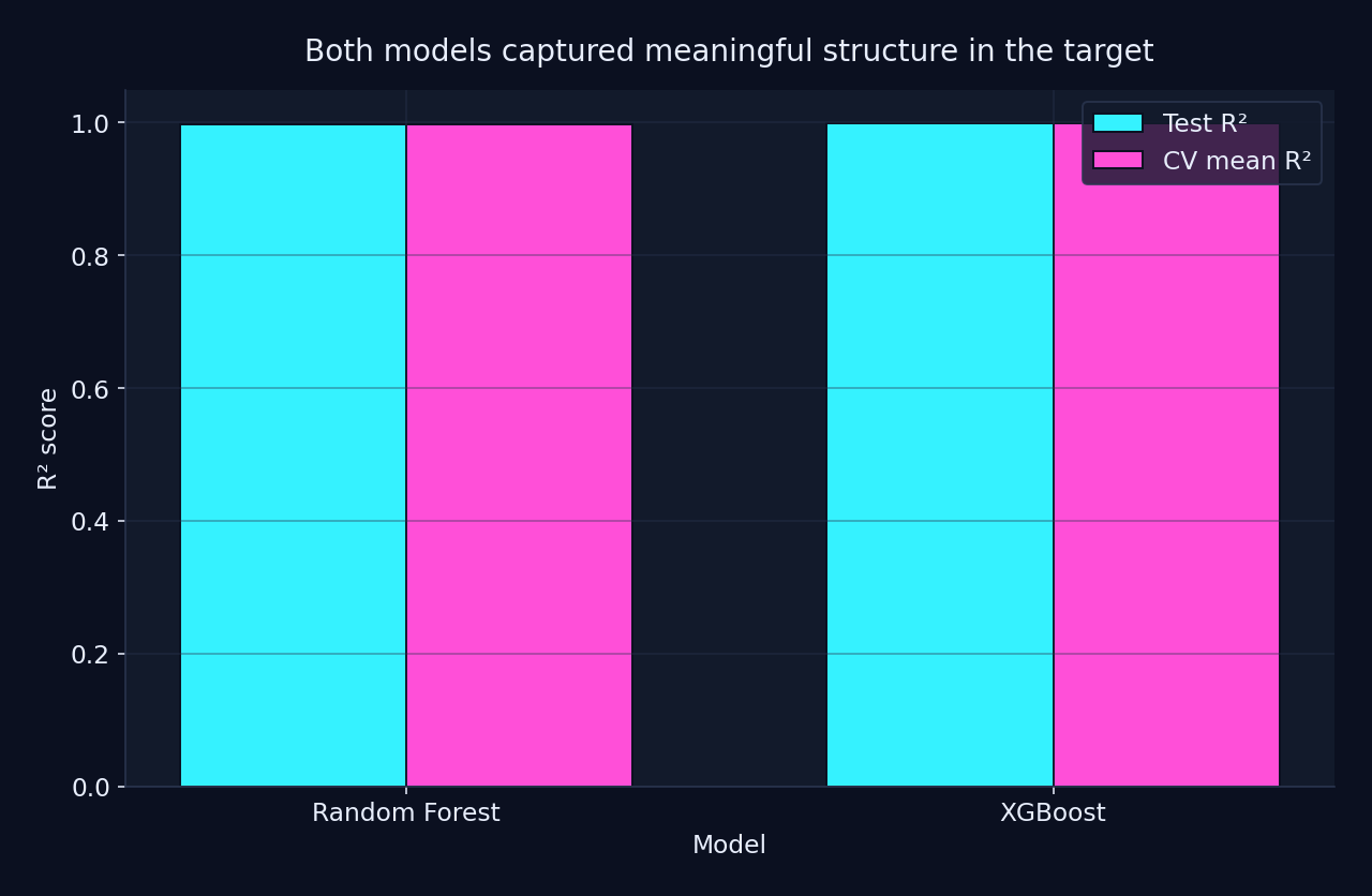
After switching to a log-transformed target, both models captured strong structure in the dataset much more consistently. I treated that as evidence that the pipeline was learning a more stable version of the proxy target, not as proof of a scientifically rigorous valuation model.

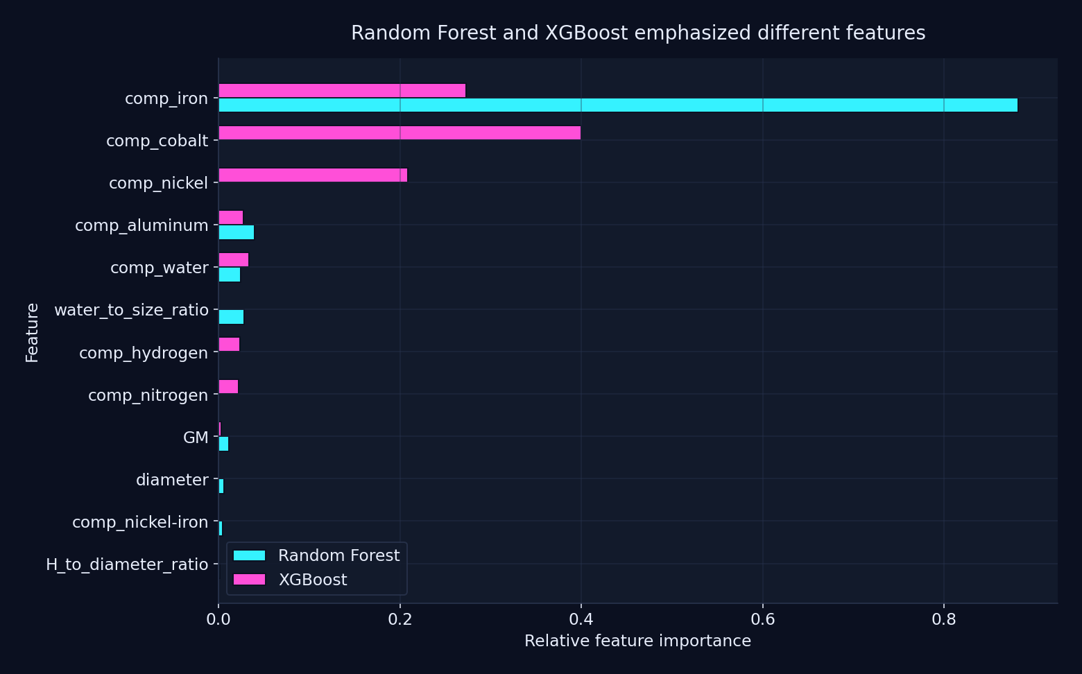
After stabilizing the target, both models concentrated much of their signal in the composition-derived features, but they still did not rank those features the same way. Random Forest leaned most heavily on estimated iron content, while XGBoost spread its importance more across iron, cobalt, and nickel-related inputs.

That difference mattered to me because it reinforced two things at once: first, the hand-built composition priors were doing a lot of work in the final pipeline, and second, even within that shared feature space, model choice still changed what looked most important.

target = np.log1p(dataset['price'].clip(lower=0))

X_train, X_test, y_train, y_test = train_test_split(
    features, target, test_size=0.2, random_state=42
)

rf_model = RandomForestRegressor(n_estimators=300, random_state=42, n_jobs=-1)
rf_model.fit(X_train, y_train)

xgb_model = XGBRegressor(
    n_estimators=400,
    max_depth=4,
    learning_rate=0.05,
    subsample=0.8,
    colsample_bytree=0.8,
    reg_lambda=1.0,
    objective='reg:squarederror',
    random_state=42,
    n_jobs=-1
)
xgb_model.fit(X_train, y_train)

This was probably the most conventional part of the project. By the time I got here, most of the interesting choices had already been made upstream in the data collection, target definition, and feature engineering. The models mattered, but the shape of the problem mattered more.

What I Found Interesting

What I found most interesting about this project was how quickly it stopped being “just an ML problem.” On the surface, it looked like a straightforward modeling exercise: collect data, clean it up, engineer some features, and train a regressor. But as soon as I started making decisions about composition, orbital structure, and what the target was supposed to represent, it became obvious that the interesting part was really in the assumptions.

I also liked how naturally this project sat at the intersection of several things I care about. My geology background makes me naturally interested in composition and material properties, while the software side let me turn that curiosity into something concrete. That combination made the project feel more personal than a generic machine learning exercise.

The feature engineering was probably the most fun part. Turning raw asteroid fields into things like total_metal, water_to_size_ratio, and orbit_stability made the dataset feel a lot more legible. Even when some of those features were rough proxies, they forced me to think about what I actually believed might matter and why.

The visualizations were also revealing. The diameter distribution made the small-object concentration obvious, while the diameter-versus-price plot showed how strongly the speculative target was dominated by size. The visible banding suggested that the pricing logic depended on more than size alone.

One thing I found especially interesting was how sensitive the modeling story was to target formulation. Once I moved from the raw price field to a log-transformed version, the results became much more stable, and even the feature importance rankings shifted. That ended up feeling like a more important lesson than the raw metric values themselves.

What Feels Shaky in Hindsight

The biggest thing that feels shaky in hindsight is the target itself. I was not modeling any rigorous notion of true asteroid economic value. I was modeling a speculative value field from a public dataset, which means the assumptions were already embedded in the target before I ever trained a model. That makes the project interesting, but it also puts a ceiling on how meaningful the results can be.

The composition mapping is another place where the project is clearly assumption-heavy. Using spectral class as a proxy for composition was a practical way to make the dataset richer, but it is still a proxy. It is not the same as directly measured composition, and the hand-built mapping I used was much closer to a rough prior than a scientifically defensible model.

Some of the engineered features also fall into that same category. A few felt reasonably grounded, while others were more heuristic than physical. That is not necessarily bad for an exploratory project, but it matters if I want to claim real understanding rather than just a working pipeline.

The other thing that feels shaky is how quickly I moved from idea to implementation. AI helped me get to something concrete much faster, which was useful, but it also made it easier to build pieces that I could describe better than I could fully justify. Looking back, I can see where I was building momentum faster than I was building understanding.

Why This Project Changed How I Want to Learn

This project changed how I want to learn because it exposed the difference between assembling a system and really understanding it. I was able to get from curiosity to a working pipeline relatively quickly, and that part was exciting. But revisiting it later made it clear that there were big pieces of the physics, data assumptions, and machine learning workflow that I wanted to understand more deeply.

AI is a great tool, but this project reminded me that if you do not understand the domain well enough, it is very easy to build something faster than you can actually support it. You can get to a working implementation, but that does not mean you can explain the assumptions behind it, debug it when it goes wrong, or maintain it with confidence later.

That does not make AI useless to me. If anything, it makes me want to use it more deliberately. I still want help moving quickly, but I want that help to act more like tutoring, explanation, and feedback instead of a shortcut to code I cannot fully defend.

In that sense, this project was valuable even beyond the model itself. It gave me something concrete to react to. It showed me what kinds of questions actually hold my attention, where my intuition is still weak, and what I want to go back and learn properly.

AI is a great tool, but this project reminded me that if you do not understand the domain well enough, it is very easy to build something faster than you can actually support it. You can get to a working implementation, but that does not mean you can explain the assumptions behind it, debug it when it goes wrong, or maintain it with confidence later.

What I’m Building Next

The next step for me is to stop treating projects like this as isolated experiments and start using them as a path into stronger foundations.

I want to go back and build up the pieces that this project made me realize I was missing: a better understanding of orbital mechanics, a more grounded grasp of machine learning fundamentals, and eventually a deeper understanding of image models and transformers.

So the next phase of this series is going to be more deliberate. Instead of jumping straight to ambitious ideas and asking AI to help me assemble them, I want to use those ideas as motivation to learn the underlying concepts more carefully. That means building smaller projects around orbital dynamics, basic ML, and model intuition before I try to return to bigger ideas like asteroid analysis systems or coordinated spacecraft.

In other words, this project was not the end goal. It was the thing that convinced me I had found a direction worth taking seriously.